Cohesive Element Pre-Stretching

As indicated in the simple 1-D test problem described above, the oscillations associated with the cohesive element insertion are linked to the amplitude of the local stress field present in the vicinity of the proposed cohesive edge at the time of the element insertion. The basic idea pursued hereafter consists in introducing the cohesive element in a manner that would minimize the perturbation on the local stress field. This goal can be accomplished by inserting the cohesive element in a pre-deformed state - either stretched or contracted depending on the tensile or compressive nature of the local stress field. In other words, the nodal oscillations will be minimized because the pre-deformed cohesive element will be in a state of separation close to the expected separation had the cohesive element been present from the beginning.

In order to apply the cohesive element pre-stretching at the time of insertion, we must determine the nodal displacement jump across the cohesive surface to be introduced. A relatively straightforward approach to accomplish this is to enforce local equilibrium on the assembly composed of the cohesive element and the adjacent volumetric element. To demonstrate this idea, let us consider the simple 1-D system shown in Figure 2.18.

Figure 2.18: 1-D cohesive element pre-stretching concept.

The local equilibrium equations for the four nodes involved in the cohesive element insertion can be written in the form:

$$[{\bf K}]\{{\bf D}\} = \{{\bf R}\} \vspace*{0.5cm}$$ (2.28)

where, for an axially loaded bar problem, the stiffness matrix $[{\bf K}]$, nodal displacement vector $\{{\bf D}\}$ and force vector $\{{\bf R}\}$ are given by

$$\left[\begin{array}{cccc} k_a & -k_a & 0 & 0 \\ -k_a & k_a+k_c & ... ..._a}^{internal} \\ 0 \\ 0 \\ {R_b}^{internal} \end{array}\right] \vspace*{0.5cm}$$ (2.29)

in which the stiffnesses $k_a$ and $k_b$ of the bar elements $a$ and $b$ are given by

$$k_a = \frac{{E_a}{A_a}}{l_a} \hspace*{2cm} k_b = \frac{{E_b}{A_b}}{l_b} \vspace*{0.5cm}$$ (2.30)

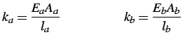
The cohesive node stiffness $k_c$ is given by

$$k_c = \frac{S_{initial}}{1-S_{initial}} \frac{\sigma_{max}}{\Delta_c} \vspace*{0.5cm}$$ (2.31)

where $S_{initial}$ is the initial strength parameter, $\sigma_{max}$ is the critical failure stress and $\Delta_c$ is the critical separation.

The nodal forces, ${R_a}^{internal}$ and ${R_b}^{internal}$ acting on nodes 1 and 3, respectively, quantify the existing stress state on volumetric elements $a$ and $b$. Prescribing the nodal displacements at nodes 1 and 3 as those computed at these nodes at the time of insertion, we can readily solve the resulting 2-by-2 linear system in terms of $u_2$ and $u_4$:

$$\left[\begin{array}{cc} k_a+k_c & -k_c \\ -k_c & k_c+k_b \\ \end{... ... = \left[\begin{array}{c} k_a u_1 \\ k_b u_3 \end{array}\right] \vspace*{0.5cm}$$ (2.32)

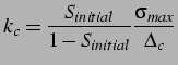
While this method is quite simple in 1-D and for a single cohesive element, it is quite more cumbersome in 2-D and where a large number of elements are inserted simultaneously. A simpler method inspired from the pre-stretching approach consists in using the local stress field directly to compute, with the aid of the traction-separation law, the initial displacement jump to be applied across the cohesive surface.

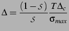
Inverting the traction-separation relation introduced earlier, the displacement jump can be written as

$${\Delta} = \frac{(1-\mathcal S)}{\mathcal S} \frac{T \Delta_c} {\sigma_{max}} \vspace*{0.5cm}$$ (2.33)

The applied cohesive traction, $T$, is simply chosen as the average of the nodal internal forces applied on nodes $2$ and $4$ by the volumetric elements a and b, respectively. As shown in Figure 2.19, the separation is then applied evenly in both directions from the current location of the original node (i.e., node $\char93 2$). This even distribution has shown to give good results although a mass-weighted separation can be used by which the displacement is greater towards the lighter edge element.

Figure 2.19: 1-D cohesive element pre-stretching concept, with the pre-stretch applied equally on the two nodes.

In two dimensions, the nodal separations can receive contributions from multiple neighboring cohesive elements, and in both the $x$ and $y$ directions. Figure 2.20 is a schematic example of three connected edges where cohesive elements are inserted. We first transform the normal and tangential cohesive separations into the separations along the principal $x$ and $y-$axes, resulting in separations of $\Delta x$ and $\Delta y$. When applying these separations to the various nodes we must be careful not to simply sum the contributions from each neighboring cohesive element. Instead we can either use the maximum or minimum nodal separation, the average of all of the neighboring separations, or some weighted distribution based on the mass of the current node. After some testing we found that the optimal approach is to use the average of the neighboring cohesive separations. The other approaches induced greater oscillations for every test case.

Figure 2.20: 2-D separation contributions from neighboring cohesive elements.

Figure 2.21 shows the effect of pre-stretching on the separation of the cohesive node for the $0th$ (0 $s$), $1000th$ ($33.3$ $s$) and $2000th$ ($66.6$ $s$) time step insertion cases for the simple 1-D problem discussed earlier. The oscillations, while still present, have been drastically reduced. More tests of the effect of adaptive cohesive element insertion on the solution are presented in Chapters $3$ and $4$.

Figure 2.21: 1-D test problem separation oscillations of nodes $2$ & $4$ (Figure 2.14) resulting from insertion with pre-stretching at time 0, $1000\Delta t$ ($33.3$ $s$), $2000\Delta t$ ($66.6$ $s$).